Tutorial 1: Engeneered Endothelin-1 peptide dimer
| Author: | Kota Kasahara |
|---|
System
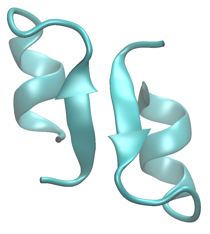
In this tutorial, we will analyze the trajectory of a MD simulation of Endothelin-1 dimer, based on PDB ID:1t7h [Hoh_2004] . The system is composed of two engineered Endothelin-1 peptides and 7,395 water molecules with 19 and 21 sodium and chrolide ions (150 mM), respectively. The total number of atoms is 22,787.
The MD simulation was perfomed using Gromacs [Pronk_2013] . The temperature and pressure of the system were kept at 300 K and 1 atm with Berendsen thermostat and barostat. The length of the trajectory is 100 ns with 10,000 snapshots.
The files for the tutorial are placed at ${MDCCTOOLS}/tutorial_files directory.
- initial.pdb
- The original PDB file
- initial_md.pdb
- The .pdb file prepared as the initial structure for the MD simulation.
- traj.trr
- The trajctory file written in the Gromacs .trr format.
| [Hoh_2004] | Hoh, F.,Cerdan, R.,Kaas, Q.,Nishi, Y.,Chiche, L.,Kubo, S.,Chino, N.,Kobayashi, Y.,Dumas, C.,Aumelas, A. High-resolution X-ray structure of the unexpectedly stable dimer of the [Lys(-2)-Arg(-1)-des(17-21)]endothelin-1 peptide, Biochemistry, 43:15154-15168, 2004 |
| [Pronk_2013] | Pronk S, Páll S, Schulz R, Larsson P, Bjelkmar P, et al. (2013) GROMACS 4.5: a high-throughput and highly parallel open source molecular simulation toolkit. Bioinformatics 29: 845–854. doi:10.1093/bioinformatics/btt055. |
Preparation
Trajectory file
Our program can read the trajectory files written in Gromacs .trr format. If you have the trajectory file in another format, it has to be converted into the .trr format. mDCC_tools include file conversion script, powered by MDAnalysis library [Michaud-Agrawal_2011]. For your information VMD plug-in [Humphrey_1996] is also useful to convert the trajectory file.
For .ncdf (AMBER) and .dcd (CHARMM, NAMD, and LAMMPS) trajectory files, the following script convert it into .trr file:
python ${MDCCTOOLS}/bin/convert_trajectory_mda.py \
  -i traj.dcd \
  --i-pdb reference.pdb \
  -o traj.trr \
  -f trr

python ${MDCCTOOLS}/bin/convert_trajectory_mda.py \
  -i traj.ncdf \
  --i-pdb reference.pdb \
  -o traj.trr \
  -f trr
For trajectory files in the PRESTO format (generated by PRESTO v3, Cosgene and, Psygene-G [Mashimo_2013] ), the other script is required:
python ${MDCCTOOLS}/bin/convert_trajectory_presto.py \
  --i-crd traj.cod \
  --i-pdb reference.pdb \
  -o traj.trr
| [Michaud-Agrawal_2011] | Michaud-Agrawal N, Denning EJ, Woolf TB, Beckstein O (2011) MDAnalysis: A toolkit for the analysis of molecular dynamics simulations. J Comput Chem 32: 2319–2327. doi:10.1002/jcc.21787. |
| [Humphrey_1996] | Humphrey W, Dalke A, Schulten K (1996) VMD: visual molecular dynamics. J Mol Graph 14: 33–8–27–8. |
| [Mashimo_2013] | Mashimo T, Fukunishi Y, Narutoshi K, Takano Y, Fukuda I, et al. (2013) Molecular Dynamics Simulations Accelerated by GPU for Biological Macromolecules with a Non-Ewald Scheme for Electrostatic Interactions. J Chem Theory Comput 9: 5599–5609. doi:10.1021/ct400342e. |
The RMS fitting should be performed for the trajecotry file because the mDCC analysis depends on the absolute position of atoms. If you use Gromacs tools,
trjconv -f traj_orig.trr -o traj_tmp.trr -pbc mol
trjconv -f traj_tmp.trr -o traj.trr -fit rot+trans
The fitted trajectory file (traj.trr) is distributed for the tutorial.
Converting the Gromacs trajectory into the mDCC original format
mDCC tools use an original file format of trajectory in order to improve file I/O in the programs. The following command converts the trajectory file, traj.trr
cp ${MDCCTOOLS}/tutorial_files/traj.trr .

python ${MDCCTOOLS}/bin/convert_trajectory.py \
  -i traj.trr \
  -o traj.trrmdcc
The –double option is required for trajectory files recording the real values in double precision.
- -i option specifies input .trr file in Gromacs format
- -o option specifies the name of output trajecotry file
The new file traj.trrmdcc will be generated.
Generating the data table
In this process, data tables for information of atoms and residues are generated. This process is required for the data visualizations with R and SQLite in the last part of this tutorial.:
cp ${MDCCTOOLS}/tutorial_files/initial_md.pdb .
cp ${MDCCTOOLS}/tutorial_files/initial.pdb .
cp ${MDCCTOOLS}/tutorial_files/segments.txt .

python ${MDCCTOOLS}/bin/get_structure_info.py \
  -i           initial_md.pdb \
  --i-orig     initial.pdb    \
  --i-mdconf   segments.txt   \
  -o           reference.pdb                  \
  --o-pdb-canoresid reference_cano.pdb        \
  --o-atom     ref_atoms.txt                  \
  --o-res      ref_res.txt                    \
  --o-chain    ref_chain.txt                  \
  --o-atom-woh ref_atoms_woh.txt              \
  --o-res-woh  ref_res_woh.txt
–i-orig and –i-mdconf are optional.
-i initial_md.pdb is the structure of simulation model in .pdb format.
–i-orig initial.pdb is the struture of the original .pdb file, without hydrogen atoms. In the case that the residue-IDs in the MD initial structure are modified from the original IDs, this setting . The residue numbers are extracted and integrated with the information in -i initial_md.pdb. This input file is optional.
–i-mdconf segments.txt is user-defined labels for segments in the structure. In this tutorial, it used for labels of the secondary structures. This file is optional.
segments.txt:
--segment ANT    0   48   LOOP
--segment AS1   49   79  SHEET
--segment AL1   80  137   LOOP
--segment AH1  138  281  HELIX
--segment BNT  282  339   LOOP
--segment BS1  340  360  SHEET
--segment BL1  361  418   LOOP
--segment BH1  419  562  HELIX
- The reserved keyword, “–segment”.
- Name for this segment (users can arbitraliry define it).
- The first atom-ID of this segment.
- The last atom-ID of this segment.
- Type of this segment (users can arbitrarily define it).
-o reference.pdb is an output .pdb file name.
–o-atom ref_atoms.txt is a table of information about atoms in the structure, written in the tab separated text.
ref_atoms.txt:
atom_id.int atom_name.string res_name.string res_id.int res_num.int \
    res_num_auth.int chain_id.string segment.string seg_type.string
0       N       LYS     0       1       1       A       ANT     LOOP
1       H1      LYS     0       1       1       A       ANT     LOOP
2       H2      LYS     0       1       1       A       ANT     LOOP
3       H3      LYS     0       1       1       A       ANT     LOOP
The first line indicates the header of each column. From the second line, each line corresponds to each atom.
- atom_id.int: Automatically assigned atom-ID beginning with zero.
- atom_name.string: The name of atom taken from initial_md.pdb.
- res_name.string: The name of residue taken from initial_md.pdb.
- res_id.int: Automatically assigned residue-ID beginning with zero.
- res_num.int: Residue number taken from initial_md.pdb.
- res_num_auth.int: Residue number taken from initial.pdb.
- chain_id.string: Chain-ID taken from initial_md.pdb
- segment.string: Segment name defined in segments.txt
- seg_type.string: Segment type defined in segments.txt
–o-res ref_res.txt is a table of information about residues in the structure, written in the tab separated text.
ref_res.txt:
res_id.int res_num.int res_num_auth.int res_name.string first_atom_id.int \
    last_atom_id.int res_label.string \
    chain_id.string segment.string seg_type.string
0       1       1       LYS     0       23      Lys1    A       ANT     LOOP
1       2       2       ARG     24      47      Arg2    A       ANT     LOOP
2       3       3       CYS     48      57      Cys3    A       ANT     LOOP
The first line indicates the header of each column. From the second line, each line corresponds to each residue.
- res_id.int: Automatically assigned residue-ID beginning with zero.
- res_num.int: Residue number taken from initial_md.pdb.
- res_num_auth.int: Residue number taken from initial.pdb.
- res_name.string: The name of residue taken from initial_md.pdb.
- first_atom_id.int: The first atom-ID of this residue.
- last_atom_id.int: The last atom-ID of this residue.
- res_label.string: The label for this residue.
- chain_id.string: Chain-ID taken from initial_md.pdb
- segment.string: Segment name defined in segments.txt
- seg_type.string: Segment type defined in segments.txt
–o-chain ref_chain.txt is a table of information about chains in the structure, written in the tab separated text.
ref_chain.txt:
chain_id.string chain_type.string first_atom_id.int last_atom_id.int \
    first_res_id.int last_res_id.int
A       PEPTIDE 0       280     0       17
B       PEPTIDE 281     561     18       35
The first line indicates the header of each column. From the second line, each line corresponds to each chain.
- chain_id.string: Chain-ID taken from initial_md.pdb
- chain_type.string: Type of the chain.
- first_atom_id.int: The first atom-ID of this chain.
- last_atom_id.int: The last atom-ID of this chain.
- first_res_id.int: The first residue-ID of this chain.
- last_res_id.int: The last residue-ID of this chain.
–o-atoms-woh ref_atoms_woh.txt is the same as –o-atom ref_atoms.txt except for absence of the first header line.
–o-res-woh ref_res_woh.txt is the same as –o-res ref_res.txt except for absence of the first header line.
–o-chain-woh ref_chain_woh.txt is the same as –o-chain ref_chain.txt except for absence of the first header line.
Pattern recognition
Execute the mdcc_learn program
mdcc_learn program performs a pattern recognition for a spatial distribution of atomic coordinates. Here, we will apply mdcc_learn for all heavy atoms. For the system consisting of Nh heavy atoms, mdcc_learn should be repeatedly executed Nh times.
Execute the commands from the shell:
mkdir mdcclearn_out
mkdir mdcclearn_bash
cp ${MDCCTOOLS}/tutorial_files/mdcclearn_conf_template.txt .
cp ${MDCCTOOLS}/tutorial_files/mdcclearn_crd.bash .
mdcc_learn_crd.bash script repeats executions of mdcc_learn program.
For example,
bash mdcclearn_crd.bash 3 1
bash mdcclearn_crd.bash 3 2
bash mdcclearn_crd.bash 3 3
Here we have 307 heavy atoms in the system, and the mdcc_learn jobs are divided into three jobs, each of them processes 102 or 103 atoms. The first argument means the total number of divided jobs, and the second means the ID of a job. They can be executed in parallel.
mdcc_learn_crd.bash:
#!/bin/bash

n_cal=${1}
id_cal=${2}

echo "${id_cal} / ${n_cal}"

fn_mdcclearn_conf="mdcclearn_conf_template.txt"
fn_mdcclearn_sh="mdcclearn_${id_cal}.bash"
fn_pdb="reference.pdb"

python ${MDCCTOOLS}/run_mdcc_tool.py \
    --mode mdcclearn \
    --pdb ${fn_pdb} \
    --select "not type H" \
    --n-div ${n_cal} \
    --task-id ${id_cal} \
    --mdcc-conf ${fn_mdcclearn_conf} \
    --mdcc-bin "${MDCCTOOLS}/bin/mdcc_learn" \
    --fn-sh mdcclearn_bash/${fn_mdcclern_sh}

cd mdcclearn_bash
bash ./${fn_mdcclearn_sh}
- –select specifies atoms to be analyzed. The syntax is defined in MDAnalysis library. See the document of MDAnalysis.
For each mdcc_learn job, the configure file is loaded.
mdcclearn_conf_template.txt:
-atom #{COLUMN}
-n-mixed-element 5
-skip-data 1
-skip-header 10
-fn-data-table  ../traj.trrmdcc
- -n-mixed-element 5 means the number of Gaussian functions to model the distribution.
- -data-skip 1 means the every frames in the trajectory are sampled. When it is 2, one of every two frames are sampled.
- -header-skip 10 means the first 10 frames are skipped. They considered as relaxation steps.
- -fn-data-table specifies the input trajectory file in our original format.
- -fn-out-gaussian specifies the output file name. The keyword #{COLUMN} is replaced into atom-ID by the python script.
The results of mdcc_learn jobs are output at mdcclearn_out direcoty. The number at the tail of file name indicates the atom-ID.
mdcclearn_out.txt.0:
0       2.0036e-07      0       0       0       0.2     0       0       0       0.2     0       0       0       0.2
1       2.0036e-07      0       0       0       0.2     0       0       0       0.2     0       0       0       0.2
2       2.0036e-07      0       0       0       0.2     0       0       0       0.2     0       0       0       0.2
3       0.00184653      21.1787 36.237  25.1603 35.3337 59.9602 41.5524 59.9602 102.601 71.1896 41.5524 71.1896 49.5847
4       0.998153        25.2273 39.9415 30.0973 0.893441        0.432562        0.228942        0.432562        0.510912        0.252169        0.228942        0.252169        0.493589
Each column indicate the parameters for each Gaussian function.
- The 1st column is ID of the Gaussian functions.
- The 2nd column is the probability.
- The 3rd-5th columns are the mean of the Gaussian in x, y, and z coordinates.
- The remaining 9 columns indicate the covariance matrix.
Integrating the results of all heavy atoms
After finishing all jobs, all the results are concatenated and global-ID for all Gaussian functions are assigned.
Execute the command from the shell:
python ${MDCCTOOLS}/bin/mdcclearn_result_summary.py \
  --dir-mdcclearn mdcclearn_out --pref-mdcclearn mdcclearn_out.txt. \
  -o crd_mdcclearn_gauss.txt \
  --min-pi 0.01
- –min-pi 0.01 means that the Gaussian funcitons probability of which is less than 0.01 will be eliminated
The files named mdcclearn_out.txt.* in the directory mdcclearn_out are merged to a single file crd_mdcclearn_gauss.txt.
Assigning the trajectory on the patterns
In the similar way to the mdcc_learn case, mdcc_assign program will be executed with dividing into some jobs.
Execute the commands from the shell:
mkdir -p mdccassign_bash/assign
cp ${MDCCTOOLS}/tutorial_files/mdccassign_conf_template.txt .
cp ${MDCCTOOLS}/tutorial_files/mdccassign_crd.bash .
bash mdccassign_crd.bash 3 1
bash mdccassign_crd.bash 3 2
bash mdccassign_crd.bash 3 3
mdccassign_crd.bash:
#!/bin/bash
n_cal=${1}
id_cal=${2}

fn_mdccassign_conf="mdccassign_conf_template.txt"
fn_mdccassign_sh="mdccassign_${id_cal}.bash"
fn_pdb="reference.pdb"

echo "${id_cal} / ${n_cal}"

python2.7 ${MDCCTOOLS}/bin/run_mdcc_tool.py \
  --mode mdccassign \
  --pdb ${fn_pdb} \
  --select "not type H" \
  --n-div ${n_cal} \
  --task-id ${id_cal} \
  --mdcc-conf ${fn_mdccassign_conf} \
  --mdcc-bin "${MDCCTOOLS}/bin/mdccassign" \
  --fn-sh mdccassign_bash/${fn_mdccassign_sh}

cd mdccassign_bash
bash ./${fn_mdccassign_sh}
- –select specifies atoms to be analyzed.
mdccassign_conf_template.txt:
-mode assign-trajtrans
-target-column #{COLUMN}
-skip-data 1
-skip-header 0
-skip-header-gaussian 1
-fn-gaussians ../crd_mdcclearn_gauss.txt
-fn-interactions  ../traj.trrmdcc
-fn-result assign/assign.dat.#{COLUMN}
-gmm-type #{COLUMN}
- The string #{COLUMN} will be replaced into the atom-ID by the python script
- -mode assign-trajtrans is a reserved keyword. It should not be changed.
- -target-column specifies the atom-ID to be processed in the job.
- -skip-header-gaussian 1 means the first line in ../crd_mdcclearn_gauss.txt will be omitted.
We will get many binary files assign.txt.* in the directory mdccassign_bash/assign.
Calculating the mDCC
The correlations of all pairs of modes, which defined with mdcc_learn program, will be calculated by using a python script cal_mdcc.py. In the same way as execution of mdcc_learn and mdcc_assign, execute the commands from the shell as following commands:
mkdir mdcc
cp ${MDCCTOOLS}/tutorial_files/cal_mdcc.bash .
bash cal_mdcc.bash 3 1
bash cal_mdcc.bash 3 2
bash cal_mdcc.bash 3 3
cat mdcc/corr.txt.* > corr_mdcc.txt
Note that this process calculate all pairs of modes, and thus the calculation time depends O(N^2).
cal_mdcc.bash:
#!/bin/bash
n_cal=${1}
id_cal=${2}

python2.7 ${MDCCTOOLS}/bin/cal_mdcc.py \
  --fn-ref reference_cano.pdb \
  --gaussian crd_mdcclearn_gauss.txt \
  --pref-assign mdccassign_bash/assign/assign.dat. \
  --fn-crd-bin  traj.trrmdcc \
  --select "not type H" \
  --o-mdcc mdcc/corr.txt.${id_cal} \
  --n-div ${n_cal} \
  --task-id ${id_cal} \
  --assign-binary \
  --range-time-begin 10
- –select “not type H” specifies the atoms to be considered. All the pairs in these atoms will be calculated. The syntax of this selection string follows MDAnalysis library (http://pythonhosted.org/MDAnalysis).
- –range-time-begin 10 means the first nine frames of the trajectory will be omitted.
We will obtain mdcc.txt.* files.
corr_mdcc.txt:
0   421 0   512 0.0672200182733 1.0 17.0161954061
0   423 0   514 0.0541268903286 1.0 15.8070676053
421 423 512 514 0.763646415298  1.0 1.29259511836
0   1   0   4   0.873601422704  1.0 1.35943704893
- The 1st and 2nd columns: IDs of modes corresponding to crd_mdcclearn_gauss.txt.
- The 3rd and 4th columns: atom-IDs (zero-origin)
- The 5th column: the mDCC correlation coefficient
- The 6th column: simultaneous probability for the two modes.
- The 7th column: the distance between ceters of the two modes.
Calculating the conventional DCC
For comparison, the conventional DCC is calculated by using the same script.
Execute the commands from the shell:
mkdir dcc
cp ${MDCCTOOLS}/tutorial_files/cal_dcc.bash .
bash cal_dcc.bash 1 1
cat dcc/corr.txt.* > corr_dcc.txt
Calculating the interatomic distance
The initial and averaged distance between atoms are calculated.
Execute the commands from the shell:
mkdir dist
cp ${MDCCTOOLS}/tutorial_files/cal_dist.bash .
bash cal_dist.bash 1 1
cat dist/dist.txt.* > dist.txt
cp ${MDCCTOOLS}/tutorial_files/dist_init.bash .
bash dist_init.bash
Gathering the data into SQLite database
The data generated in the previous processes is gatered into a relational database.
First, remove the first line (column headers) from the crd_mdcclearn_gauss.txt file.
vi crd_mdcclearn_gauss.txt
SQL queries are in the files sqlquery_*.sql. The bash file exe_sql.bash executes the queries and ouput some files for following analyses.
mkdir sqlite
cd sqlite
cp ${MDCCTOOLS}/tutorial_files/*sql* .
bash exe_sql.bash
The four tab-separated tables are obtained.
- atom_atom.txt
- atom_atom_d5_c50.txt
- res_res.txt
- res_res_d5_c50.txt
Each row records information on a pair of atoms or residues. The files with “_d5_c50” is a subset of the other file, including only pairs that their distance is less than 5.0 Å and their correlation is higher than 0.5.
- res_num1.int The ID of first residue.
- res_num2.int The ID of sedond residue.
- atom_id1.int The ID of first atom.
- atom_id2.int The ID of second atom.
- gauss_id1.int The ID of the first Gaussian function.
- gauss_id2.int The ID of the second Gaussian function.
- correlation.float mDCC values between gauss_id1 and gauss_id2.
- coef.float The joint probability.
- dist.float The distance between centers of gauss_id1 and gauss_id2.
- corr_dcc.float The conventional DCC value between atom_id1 and atom_id2.
- dist_ave.float The averaged distance between the atoms.
- dist_sd.float The standard deviation of the interatomic distance.
- dist_min.float The minimum distance between these atoms.
- dist_max.float The maximum distance between these atoms.
- dist_init.float The initial distance between these atoms.
Visualizing the data with R
The R software is used for generating figures of the correlation map.
Execute the commands from the shell in the sqlite directory:
cp ${MDCCTOOLS}/tutorial_files/r_mdcc.r .
R --vanilla --slave < r_mdcc.r
The file mdcc_diff_heatmap.png will be generated.
Network analysis
The betweenness values can be calculated by the python script.
Execute the commands from the shell in the sqlite/ directory:
python ${MDCCTOOLS}/bin/nx_centrality.py \
  -i res_res_d5_c50.txt \
  --i-elem ../ref_res.txt \
  --key-elem res_id \
  -o res_cent_btw_d5_c50.txt \
  --btw
res_cent_btw_d5_c50.txt is a tab-separated table. Each row indicates each residue.
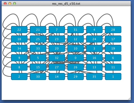
The files res_res_d5_c50.txt and res_cent_btw_d5_c50.txt can be loaded with Cytoscape software for analysis.
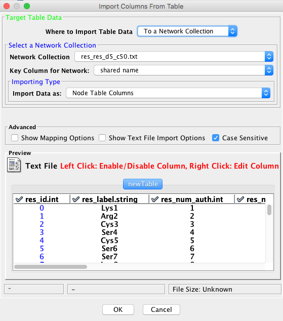
- Open the file res_res_d5_c50.txt from the menu [File] => [Import] => [Network] => [File]
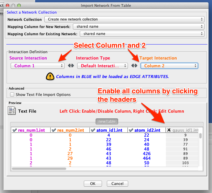
- Open the file res_cent_btw_c5_d50.txt from the menu [File] => [Import] => [Table] => [File]
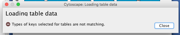
If you get the error message “Types of keys selected for tables are not matching”, specify the type of the first column “res_id.int” as “String” by right-click on the column header.
- Remove the self-loops from the menu [Edit] => [Remove Self-loops]
- Representation of the graph can be modified from the left panel.
- Choose “Style” tab at the top of the panel.
- In “Node” pane, label on each node can be specified by clicking the row “Label”. Here, we choose “res_label.string” as Column, “Passthrough Mapping” as “Mapping Type”. See the document of Cytoscape for details.
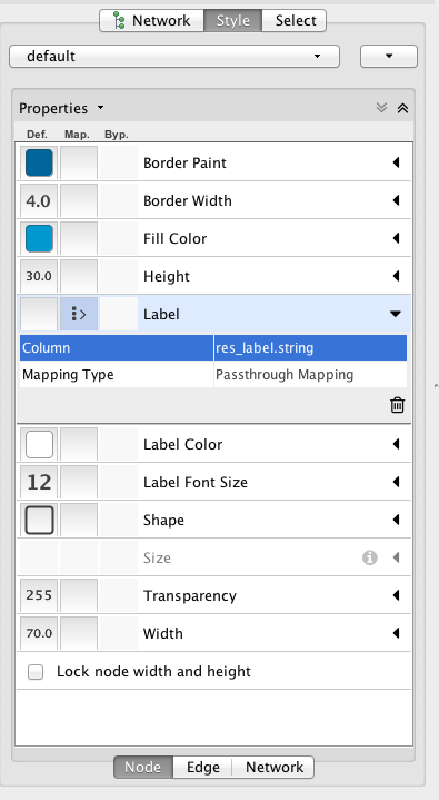
- Layout can be modified from the menu [Layout]
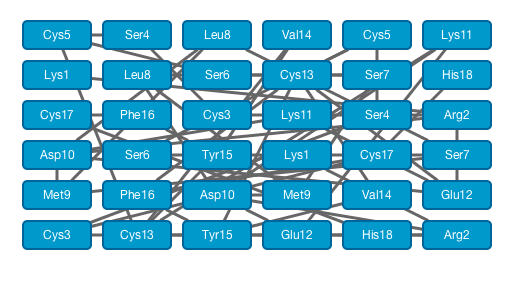
- Here we choose the circle layout.
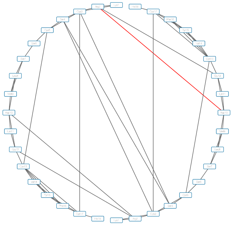
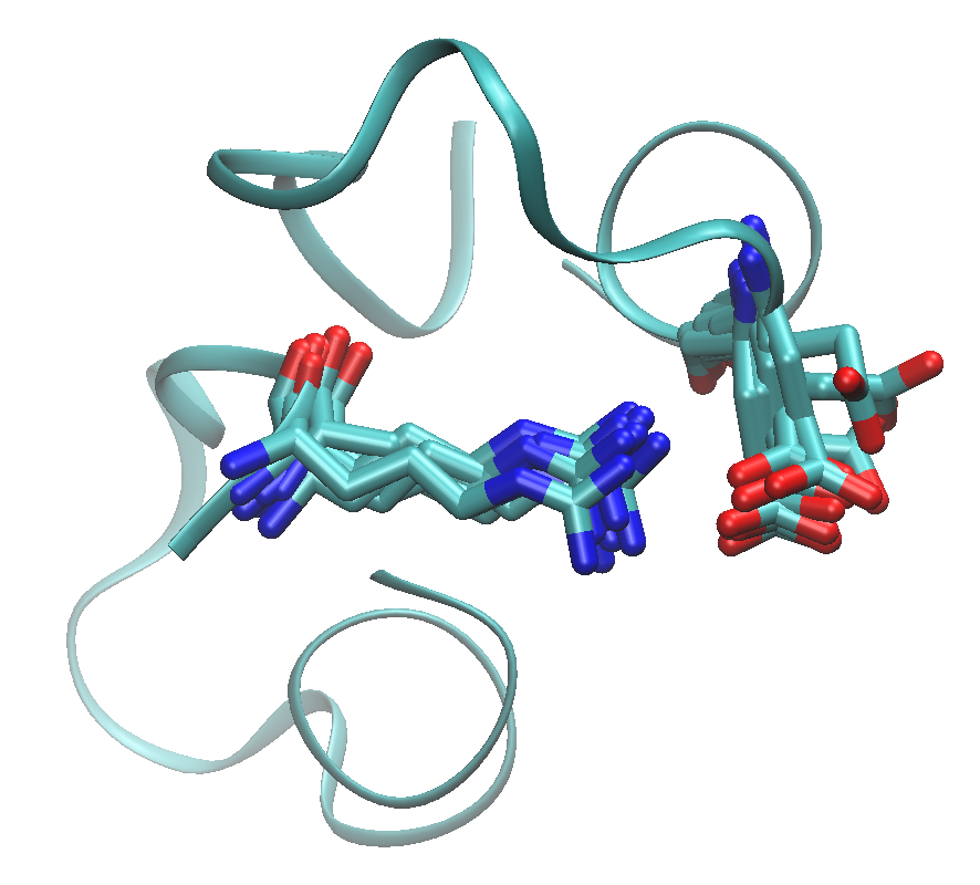
The edge between Asp10 of A chain and Arg2 in B chain is drawn as red in the figure. The DCC and mDCC values of this edge are 0.31 and 0.55, respectively. mDCC value indicates the highest correlation value in all pairs of modes between these residues. This result means that at least one of these residues shows multi-modal motion, and the interaction between them is transient. The structures of the system along the trajectory show side-chain flipping of Asp10 of A chain.
About computation times
For your information, the computation times required for this tutorial, with 290 heavy atoms, are,
- mdcc_learn ... 1,213 seconds
- mdcc_assign ... 13 seconds
- cal_mdcc ... 2,575 seconds
Only 1 core of Intel(R) Xeon(R) CPU E5-2670 was used.