Tutorial 2: Artificial 1D data
| Author: | Kota Kasahara |
|---|
The mDCC analysis method can be generalized for analyses of any multi-dimensional numerical data. In this tutorial, we will re-purpose the mDCC analysis method for non-MD application, by using a simple, artificial data.
Preparation
Artificial data
The two time series of 1D data, v0 and v1, will be generated, by using R.
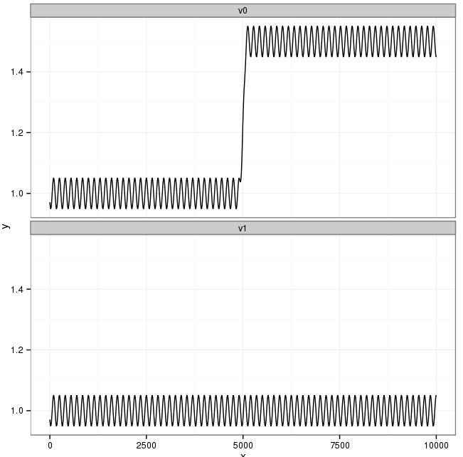
The data v0 is composed of three sine curves: 1) the first half, 2) the last half, and 3) the middle of them. The phases of the sine functions 1 and 2 are opposite. The function 3 is needed for smoothly concatenating these two functions. The data v1 is a single sine function, which is same as the first half of v0. Thus, the first half of v0 is positively correlated with v1, and the last half is negatively correlated with v1.
To generate the data table, execute the following commands on R:
gen.sin <- function(A, B, L, x){
  A * sin( B + 2*pi/L * x)
}
steps <- 1:10000
v01 <- gen.sin(0.05, 10, 150, steps) + 1
v02 <- gen.sin(-0.05, 10, 150, steps) + 1.5
grad <- (gen.sin(1,  0, 400, 1:400) + 1)[101:300]/2
w01 <- c(rep(1,4900), grad, rep(0,4900))
w02 <- 1-w01
v0 <- v01*w01 + v02 * w02
v1 <- gen.sin(0.05, 10, 150, steps) + 1
dat <- data.frame(v0, v1)
write.table(dat, "dat.txt", quote=F)
dat.txt is tab separated table:
v0 v1
1 0.971065970962453 0.971065970962453
2 0.969383757588155 0.969383757588155
3 0.967755255506516 0.967755255506516
4 0.966183321663557 0.966183321663557
..
Converting the tab separated table into the mDCC original format
The data table should be converted into the original binary file:
python ${MDCCTOOLS}/bin/convert_trajectory.py \
  -i dat.txt \
  --i-format tsv \
  -o traj.trrmdcc \
  --ignore-col 1 \
  --ignore-row 1 \
  --dim 1
- -i option specifies the input data table.
- –i-format option indicates the data format of -i file. It should be “tsv” or “trr”.
- -o option indicates the output file name.
- –ignore-col, –ignore-row options indicate how many columns and rows are skipped in the -i tsv table, respectively.
- –dim option specifies dimension of the data.
Pattern recognition
Execute the mdcc_learn program
mdcc_learn program will be executed two times. One is for the entity v0, and the other is for v1.
The input files for v0 is:
-feature 1 0 x
-n-mixed-element 5
-fn-data-table  traj.trrmdcc
-format-data-table mdcc
-fn-out-gaussian mdcclearn_out.txt.0
The other is:
-feature 1 1 x
-n-mixed-element 5
-fn-data-table  traj.trrmdcc
-format-data-table mdcc
-fn-out-gaussian mdcclearn_out.txt.1
- -fn-data-table specifies the file name of the trajectory data.
- -format-data-table specifies the file format of –fn-data-table. It should be “mdcc” or “tsv”
- -fn-out-gaussian specifies the output file name. This file describes the inferred Gaussian mixture parameters.
- -feature requires three arguments.
- The first is always 1. This field will be used for future developments.
- The second specifies 0-origin ID of entity (atom) in the data file.
- The third is the name of this feature. Any string is acceptable.
- -n-mixed-element is the number of Gaussian functions in the Gaussian mixture model.
Then, mdcc_learn is executed from the linux shell:
${MDCCTOOLS}/bin/mdcc_learn -fn-cfg mdcclearn_v0.cfg
${MDCCTOOLS}/bin/mdcc_learn -fn-cfg mdcclearn_v1.cfg
Integrating the results of all heavy entities
After that, the results of these two entities are concatenated and global-ID for all Gaussian functions are assigned.
Execute the command from the shell:
python ${MDCCTOOLS}/bin/mdcclearn_result_summary.py \
  --dir-mdcclearn ./ \
  --pref-mdcclearn mdcclearn_out.txt. \
  -o crd_mdcclearn_gauss.txt \
  --dim 1 --min-pi 0.01
- –min-pi 0.01 means that the Gaussian funcitons probability of which is less than 0.01 will be eliminated
The files named mdcclearn_out.txt.* in the directory are merged to a single file crd_mdcclearn_gauss.txt.
Assigning the trajectory on the patterns
Next, mdcc_assign is executed for the two entity, by using the following settings
mdccassign_v0.cfg:
-mode assign-mdcctraj
-target-column 0
-skip-header-gaussian 1
-fn-gaussians crd_mdcclearn_gauss.txt
-fn-data-table  traj.trrmdcc
-fn-result assign.dat.0
-gmm-type 0
-format-output binary
mdccassign_v1.cfg:
-mode assign-mdcctraj
-target-column 1
-skip-header-gaussian 1
-fn-gaussians crd_mdcclearn_gauss.txt
-fn-data-table  traj.trrmdcc
-fn-result assign.dat.1
-gmm-type 1
-format-output binary
- -mode specifies “assign-mdcctraj” or “assign-table”. The latter is for .tsv input file.
- -target-column indicates the 0-origin ID of entity (atom) in the input data file.
- -skip-header-gaussian specifies the number of lines to be skipped in the Gaussian definition file (-fn-gaussians)
- -fn-gaussians specifies the file name of Gaussian definition file obtained from the previous step.
- -fn-result specifies the file name of output.
- -gmm-type specifies the ID of Gaussian mixture, corresponding to the second column in -fn-gaussians.
Execute the commands from the shell:
${MDCCTOOLS}/bin/mdcc_assign -fn-cfg mdccassign_v0.cfg
${MDCCTOOLS}/bin/mdcc_assign -fn-cfg mdccassign_v1.cfg
Calculating the mDCC and DCC
mDCC and DCC should be calculated as following commands.
For mDCC:
python2.7 ${MDCCTOOLS}/bin/cal_mdcc.py \
  --gaussian crd_mdcclearn_gauss.txt \
  --pref-assign assign.dat. \
  --suff-assign "" \
  --o-mdcc mdcc.txt \
  --min-corr 0.0 \
  --select-id 0-1 \
  --fn-crd-bin traj.trrmdcc \
  --assign-binary
For DCC:
python2.7 ${MDCCTOOLS}/bin/cal_mdcc.py \
  --o-dcc dcc.txt \
  --min-corr 0.0 \
  --select-id 0-1 \
  --fn-crd-bin traj.trrmdcc
- –select-id specifies the 0-origin entity ID, which are analyzed. The range of IDs should be specified by concatenating the first and last IDs with ‘-‘. Or, the IDs and the range of IDs can be enumerated by sepalation with ‘,’, e.g., “1-10,12,14,16-18”.
- –pref-assign, –suff-assign indicates prefix and suffix of mdcc_assign output files. The file must be named with the prefix, IDs of elements, and suffix, e.g., “prefix.0.suffix”, “prefix.1.suffix”, ...
- –assign-binary is required for the binary mdcc_assign output.
- –o-mdcc, –o-dcc are the output file name.
- –fn-crd-bin is the input binary file.
- –min-corr indicates the minimum correlation coefficient for output.
Results
crd_mdcclearn_gauss.txt:
gc_id.int element_id.int pi.float mu1.float sigma11.float
0       0       0.496002        1.49895 0.00199557
1       0       0.49639 1.00054 0.00170489
2       1       1       0.99981 0.00145084
The mdcc_learn program found two and one Gaussian functions for the data v0 and v1, respectively.
mdcc.txt:
0       2       0       1       -0.90211646445  0.500272653972  0.499140297242
1       2       0       1       0.875547919424  0.499727346028  0.000772943337186
- The 1st and 2nd columns indicate the pair Gaussian IDs.
- The 3rd and 4th columns indicate the element IDs.
- The 5th column indicates the mDCC value.
- The 6th column indicates the simultaneous probability for the Gaussians.
- The 7th column indicates the distance between the means of the Gaussian functions.
dcc.txt:
0 1 0.00363216 0.24999
- The 1st and 2nd columns indicate the pair of element IDs.
- The 3rd column indicates the DCC value.
- The 4th column indicates the distance between the means.
As we expected, these results say that v1 positively correlated with the Gaussian 1 of v0, but it negatively correlated with the Gaussian 0 of v0. On the other hand, the conventional DCC shows no correlation between v0 and v1.
With this protocol, any kinds of multi-dimensional numerical data can be analyzed by using this tool kit.